Naive Bayes Classifier in Machine Learning

Machine Learning

Mathematical explanation and python implementation using sklearn

Naive Bayes Classifier

Naive Bayes Classifiers are probabilistic models that are used for the classification task. It is based on the Bayes theorem with an assumption of independence among predictors. In the real-world, the independence assumption may or may not be true, but still, Naive Bayes performs well.

Topics covered in this story

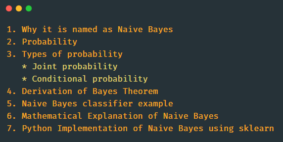
Why is it named Naive Bayes?

Naive → It is called naive because it assumes that all features in the dataset are mutually independent.
Bayes, → It is based on Bayes Theorem.

Bayes Theorem

First, let’s learn about probability.

Probability

A probability is a number that reflects the chance or likelihood that a particular event will occur.

Event → In probability, an event is an outcome of a random experiment.

P(A)=n(A)/n(S)

P(A) → Probability of an event A
n(A) →Number of favorable outcomes
n(S) →Total number of possible outcomes

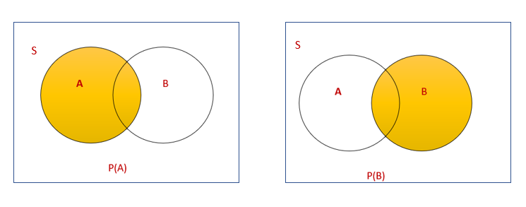
Example

P(A) → Probability of drawing a king
P(B) →Probability of drawing a red card.

P(A) =4/52
P(B)=26/52

 

Types of probability

1. Joint probability
2. Conditional probability

1. Joint Probability

A joint probability is the probability of two events occurring simultaneously.

P(A∩B) →Probability of drawing a king, which is red.

P(A∩B)=P(A)*P(B)=(4/52)*(26/52)=(1/13)*(1/2)=1/26

 

2. Conditional Probability

Conditional probability is the probability of one event occurring in the presence of a second event.

Probability of drawing a king given red → P(A|B)

 

Probability of drawing a red card given king P(B|A)

P(B|A) =P(A∩B)/P(A)

 

Derivation of Bayes Theorem

 

Naive Bayes Classifier Example

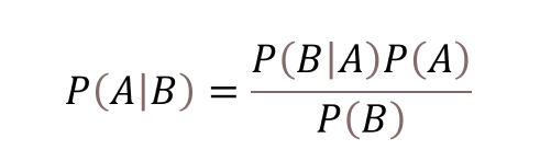
Bayes theorem is an extension of conditional probability. By using Bayes theorem, we have to use one conditional probability to calculate another one.

To calculate P(A|B), we have to calculate P(B|A) first.

Example:

If you want to predict if a person has diabetes, given the conditions? P(A|B)
Diabetes → Class → A
Conditions → Independent attributes → B

To calculate this using Naive Bayes,

1. First, calculate P(B|A) → which means from the dataset find out how many of the diabetic patient(A) has these conditions(B). This is called likelihood ratio P(B|A)
2. Then multiply with P(A) →Prior probability →Probability of diabetic patient in the dataset.
3. Then divide by P(B) → Evidence. This is the current event that occurred. Given this event has occurred, we are calculating the probability of another event that will also occur.

This concept is known as the Naive Bayes algorithm.

P(B|A) → Likelihood Ratio
P(A) → Prior Probability
P(A|B) → Posterior Probability
P(B) → Evidence

---

Dataset

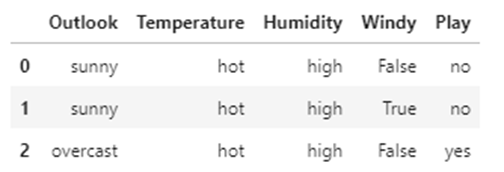
I have taken the golf dataset.

 

Consider the problem of playing golf. Here in this dataset, Play is the target variable. Whether we can play golf on a particular day or not is decided by independent variables Outlook, Temperature, Humidity, Windy.

Mathematical Explanation of Naive Bayes

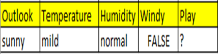
Let’s predict given the conditions sunny, mild, normal, False → Whether he/she can play golf?

 

Simplified Bayes theorem

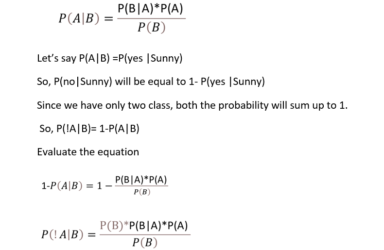
P(A|B) and P(!A|B) is decided only by the numerator value because the denominator is the same in both the equation.

So, to predict the class yes or no, we can use this formula P(A|B)=P(B|A)*P(A)

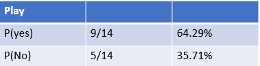
1. Calculate Prior Probability
   Out of 14 records, 9 are yes. So P(yes)=9/14 and P(no)=5/14

 

2. Calculate Likelihood Ratio

Outlook

Out of 14 records, 5-Sunny,4-Overcast,5-Rainy.

Find the probability of the day being sunny given he/she can play golf?

From the dataset, the number of sunny days we can play is 2. The total no of days we can play is 9.

So P(Sunny | yes) =2/9

Similarly, we have to calculate all variables.

 

Temperature

 

Humidity

 

Windy

 

Let’s predict given the conditions sunny, mild, normal, False → Whether he/she can play golf?

A=yes
B=(Sunny,Mild,Normal,False)

P(A|B)=P((yes)|(Sunny,Mild,Normal,False)

P(A|B)=P(B|A)*P(A)

P(yes|(Sunny,Mild,Normal,False))= P((Sunny,Mild,Normal,False)|yes) *P(yes)

[Probaility of independent events is calculated by multiplying the probability of all the events. Naive Bayes algorithm treats all the variables as independent variables)

=P(Sunny | yes)*P(Mild | yes)*P(Normal | yes)*P(False | yes)*P(yes)

=2/9 *4/9 *6/9 *6/9 *9/14

P(yes|(Sunny,Mild,Normal,False))= 0.0282

Let’s now calculate P(no|(Sunny,Mild,Normal,False))

P(no|(Sunny,Mild,Normal,False))= P((Sunny,Mild,Normal,False)|no) *P(no)

=P(Sunny | no) * P(Mild | no) * P(Normal | no) * P(False | no) * P(no)

=3/5 *2/5 *1/5 *2/5 *5/14

P(no|(Sunny,Mild,Normal,False))= =0.0068

Since 0.0282 > 0.0068[P(yes|conditions)>P(no|conditions) , for the given conditions Sunny,Mild,Normal,False , play is predicted as yes.

---

Let’s build the NB model using the same dataset

Python Implementation of Naive Bayes using sklearn

1. Import the libraries

import numpy as np
import pandas as pd
import seaborn as sns
import matplotlib.pyplot as plt

2. Load the data

df=pd.read_csv("golf_df.csv")
df.head(3)

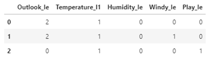
3. Converting categorical variables(string data types) to continuous variables

from sklearn.preprocessing import LabelEncoder
le=LabelEncoder()
Outlook_le=le.fit_transform(df.Outlook)
Temperature_le=le.fit_transform(df.Temperature)
Humidity_le=le.fit_transform(df.Humidity)
Windy_le=le.fit_transform(df.Windy)
Play_le=le.fit_transform(df.Play)

df["Outlook_le"]=Outlook_le
df["Temperature_l1"]=Temperature_le
df["Humidity_le"]=Humidity_le
df["Windy_le"]=Windy_le
df["Play_le"]=Play_le
df.head(3)

4. Now drop the old categorical columns from the dataframe

df=df.drop(["Outlook","Temperature","Humidity","Windy","Play"],axis=1)
df.head(3)

5. Assign x (independent variables) and y (dependent variable)

x=df.iloc[:,0:4]
x.head(3)

y=df.iloc[:,4:]
y.head(3)

6. Split data into train and test

from sklearn.model_selection import train_test_split
x_train,x_test,y_train,y_test=train_test_split(x,y,test_size=0.3,random_state=10)

7. Model building with sklearn

from sklearn.naive_bayes import GaussianNB
model=GaussianNB()
model.fit(x_train,y_train)

GaussianNB()

8. Accuracy Score

y_predict=model.predict(x_test)
from sklearn.metrics import accuracy_score
accuracy_score(y_test,y_predict,normalize=True)

Output: 1.0

9. Let’s predict the class(yes or no)given the conditions sunny, mild, normal, False.

model.predict([[2,2,1,0]])

Output: array([1])

1 → indicates yes.

So given the conditions sunny, mild, normal, False → play is yes.
So we can play golf given the conditions are sunny, mild, normal, False.

---

Github link

The code and dataset used in this story can be downloaded as a jupyter notebook from my Github link.

Conclusion

Naive Bayes classifier performs very well compared to other models when the assumption of independent predictors holds. It is very fast in both training and testing data. In some rare events, if a category which we are predicting is not observed in training data means, then the model will add zero probability and will be unable to make a prediction. To solve this, smoothing techniques like Laplace estimation is used.

My other blogs on Machine learning

Linear Regression in Python

Logistic Regression in Python

Understanding Decision Trees in Machine Learning

An Introduction to Support Vector Machine

An Introduction to K-Nearest Neighbors Algorithm

---

I hope that you have found this article helpful. Thanks for reading!