Understanding Decision Trees in Machine Learning

The math behind decision trees and how to implement them using Python and sklearn

---

Decision Trees

The decision tree is a type of supervised machine learning that is mostly used in classification problems.

The decision tree is basically greedy, top-down, recursive partitioning. “Greedy” because at each step we pick the best split possible. “Top-down” because we start with the root node, which contains all the records, and then will do the partitioning.

Root Node →The topmost node in the decision tree is known as the root node.
Decision Node→ The subnode which splits into further subnodes is known as the decision node.
Leaf/Terminal Node →A node that does not split is known as a leaf node/terminal node.

---

Data Set

 

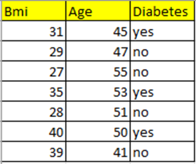
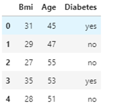
I have taken a small data set that contains the features BMI and Age and the target variable Diabetes.

Let’s predict if a person of a given age and BMI will have diabetes or not.

---

Data Set Representation

 

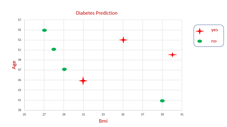
We can’t draw a single line to get a decision boundary. We are splitting the data again and again to get the decision boundary. This is how the decision tree algorithm works.

 

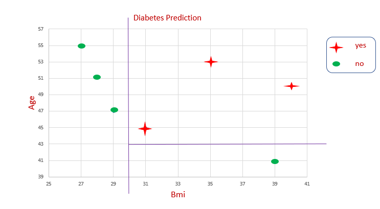
This is how partitioning happens in the decision tree.

---

Important Terms in Decision Tree Theory

Entropy

Entropy is a measure of randomness or uncertainty. Entropy level ranges between o and 1. If entropy is 0, it means this is a pure subset (no randomness). If entropy is 1, it means high randomness. Entropy is denoted by H(S).

Formula

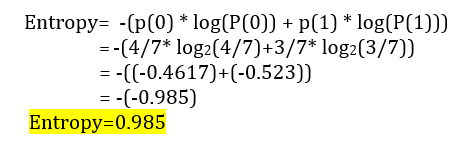
Entropy = -(p(0) * log(P(0)) + p(1) * log(P(1)))

P(0) → Probability of class 0

P(1) → Probability of class 1

---

Relationship Between Entropy and Probability

 

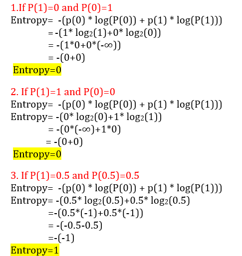
If entropy is 0, it means this is a pure subset (no randomness) (either all yes or all no). If entropy is 1, it means high randomness

Let’s plot a graph P(1)-Probability of Class 1 vs. Entropy.

From the above explanation, we know that
If P(1) is 0, Entropy =0
If P(1) is 1, Entropy =0
If P(1) is 0.5,Entropy =1

 

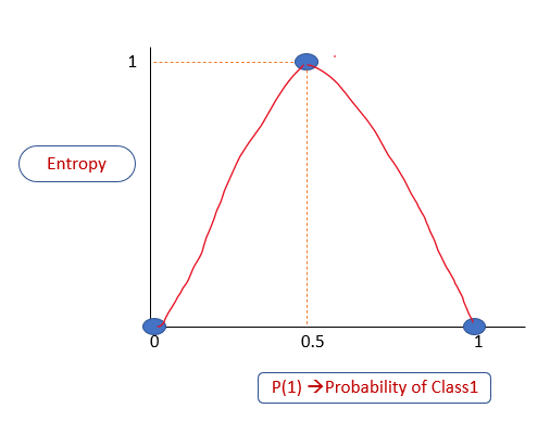
The entropy level always ranges between 0 and 1.

---

Information Gain

Information gain is calculated for a split by subtracting the weighted entropies of each branch from the original entropy. We will use it to decide the ordering of attributes in the nodes of a decision tree.

 

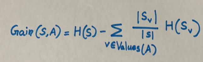
H(S) → Entropy
A →Attribute
S →Set of examples {x}
V →Possible values of A
Sv →Subset

---

How Does a Decision Tree Work?

In our data set, we have two attributes, BMI and Age. Our sample data set has seven records.

Let’s start building a decision tree with this data set.

Step 1. Root node

In the decision tree, we start with the root node. Let’s take all the records (seven in our given data set) as our training samples.

 

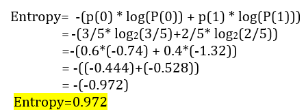
It has three yes and four no.
The probability of class 0 is 4/7. Four out of seven records belong to class 0
P(0)=4/7
The probability of class 1 is 3/7. Three out of seven records belong to class 1.
P(1)=3/7

Calculate the Entropy of the root node

 

Step 2. How does splitting occur?

We have two attributes BMI and Age. Based on these attributes, how does splitting occur? How do we check the effectiveness of the split?

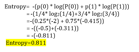
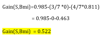
1. If we select attribute BMI as the splitting variable and ≤30 as the splitting point, we get one pure subset.

[Splitting point is considered at each data point in the dataset. So if the data points are unique, there will be n-1 split points for n data points. So depending on which splitting variable and splitting point, we get high information gain, that split is selected. If it is a large dataset, it is common to consider only split points at certain percentiles like (10%,20%,30%)of the distribution of values Since it’s a small dataset, by seeing the data points, I have selected ≤30 as the split point.]

 

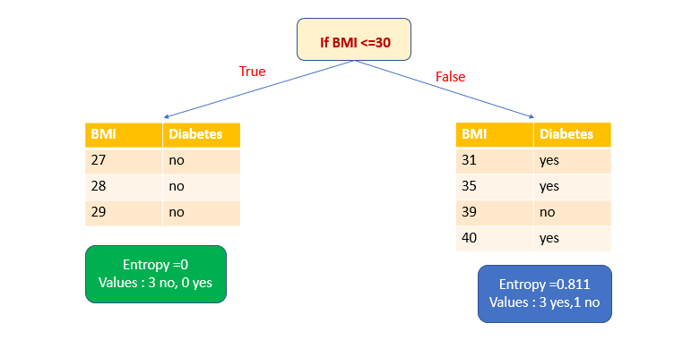
The entropy of pure subset=0.

Let’s calculate the entropy of the other subset. Here we get three yes and one no.
P(0)=1/4 [one out of four records)
P(1)=3/4 [three out of four records)

 

We have to calculate the information gain to decide which attribute to chose for splitting.

 

2. Let’s select the attribute Age as the splitting variable and ≤45 as the splitting point.

 

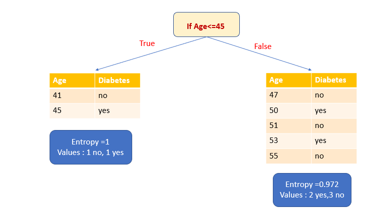
First, let’s calculate the entropy of the True subset. It has one yes and one no. It means a high level of uncertainty. The entropy is 1.

Let’s calculate the entropy of the False subset. It has two yes and three no.

 

Let’s calculate the information gain.

 

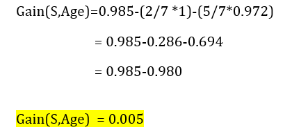
We have to choose the attribute which has high information gain. In our example, only the BMI attribute has high information gain. So the BMI attribute is chosen as the splitting variable.

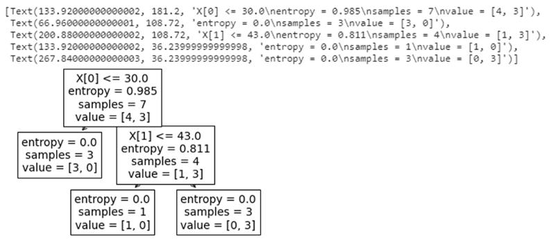
After splitting by the attribute BMI, we get one pure subset (leaf node) and one impure subset. Let’s split that impure subset again based on the attribute Age. Then we have two pure subsets (leaf node).

 

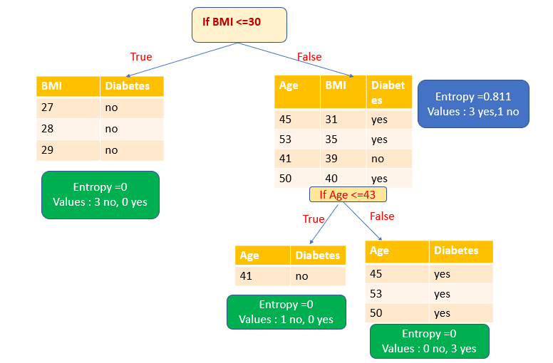
Now we have created a decision tree with pure subsets.

---

Python Implementation of a Decision Tree Using sklearn

1. Import the libraries.

import numpy as np
import pandas as pd
import matplotlib.pyplot as plt
import seaborn as sns

2. Load the data.

df=pd.read_csv("Diabetes1.csv")
df.head()

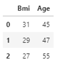
3. Split x and y variables.

The BMI and Age attributes are taken as the x variable.
The Diabetes attribute (target variable) is taken as the y variable.

x=df.iloc[:,:2]
y=df.iloc[:,2:]

x.head(3)

y.head(3)

4. Model building with sklearn

from sklearn import tree
model=tree.DecisionTreeClassifier(criterion="entropy")
model.fit(x,y)

Output: DecisionTreeClassifier (criterion=“entropy”)

5. Model score

model.score(x,y)

Output: 1.0

(Since we took a very small data set, the score is 1.)

6. Model prediction

Let’s predict whether a person of Age 47, BMI 29 will have diabetes or not. The same data is there in the data set.

model.predict([[29,47]])

Output: array([‘no’], dtype=object)

The prediction is no, which is the same as in the data set.

Let’s predict whether a person of Age 47, BMI 45 will have diabetes or not. This data is not in the data set.

model.predict([[45,47]])

Output: array([‘yes’], dtype=object)

Predicted as yes.

7. Visualize the model

tree.plot_tree(model)

---

GitHub Link

The code and data set used in this article are available in my GitHub link.

My other blogs on Machine learning

Linear Regression in Python

Logistic Regression in Python

Naive Bayes Classifier in Machine Learning

An Introduction to Support Vector Machine

An Introduction to K-Nearest Neighbors Algorithm

---

I hope that you have found this article helpful. Thanks for reading!