Central Limit Theorem — Clearly Explained

Sampling Distributions, Standard Error

Central Limit Theorem

Central Limit Theorem is one of the important concepts in Inferential Statistics. Inferential Statistics means drawing inferences about the population from the sample.

When we draw a random sample from the population and calculate the mean of the sample, it will likely differ from the population mean due to sampling fluctuation. The variation between a sample statistic and population parameter is known as sampling error.

Due to this sampling error, it may be difficult to draw inferences about population parameter from sample statistics. Central Limit Theorem is one of the important concepts in inferential statistics, which helps us to draw inferences about the population parameter from sample statistic.

Let us learn about the central limit theorem in detail in this article.

Refer to my story of Inferential Statistics — to know the basics of probability and probability distributions

---

Table of content

1. Statistic, Parameter
2. Sampling Distribution
3. Standard Error
4. Sampling Distribution Properties
5. Central Limit Theorem
6. Confidence Interval
7. Visualizing Sampling distribution

---

What are Statistic and Parameter?

Statistic → The values which represent the characteristics of the sample known as Statistic.

Parameter → The values which represent the characteristics of the population known as Parameter. (The values which we infer from statistic for the population)

Statistic →Sample Standard Deviation S, Sample Mean X

Parameter →Population Standard Deviation σ, Population Mean μ

We draw inferences from statistic to parameter.

Sampling distribution

Sampling → It means drawing representative samples from the population.

Sampling Distribution → A sampling distribution is the distribution of all possible values of a sample statistic for a given sample drawn from a population.

Sampling distribution of mean is the distribution of sample means for a given size sample selected from the population.

Steps in Sampling Distribution:

• We will draw random samples(s1,s2…sn) from the population.
• We will calculate the mean of the samples (ms1,ms2,ms2….msn).
• Then we will calculate the mean of the sampling means. (ms)

ms=(ms1+ms2+…msn)/n

n →sample size.

[Now we have calculated the mean of the sampling mean. Next, we have to calculate the standard deviation of the sampling mean]

Standard Error

Variability of sample means in the sampling distribution is the Standard Error. The standard deviation of the sampling distribution is known as the Standard Error of the mean.

Standard Error of mean = Standard deviation of population/sqrt(n)

n- sample size

[Standard error decreases when sample size increases. So large samples help in reducing standard error]

Sampling Distribution Properties.

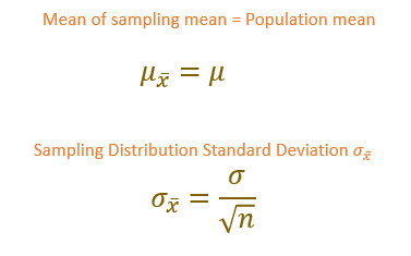
1. The mean of the sampling mean is equal to the population mean.

[When we draw many random samples from the population, the variations will cancel out. So, the mean of sampling mean equals to population mean]

2. Standard Deviation of Sampling Distribution is equal to the standard deviation of population divided by the square root of the sample size.

 

Central Limit Theorem

Central Limit Theorem states that even if the population distribution is not normal, the sampling distribution will be normally distributed if we take sufficiently large samples from the population.[ For most distributions, n>30 will give a sampling distribution which is nearly normal]

Sampling distribution properties also hold good for the central limit theorem.

Confidence Interval

We can say that the population mean will lie between a certain range by using a confidence interval.

Confidence Interval is the range of values that the population parameter can take.

Confidence Interval of Population Mean= Sample Mean + (confidence level value ) * Standard Error of the mean

Z → Z scores associated with the confidence level.

Mostly used confidence level

99% Confidence Level → Z score = 2.58
95% Confidence Level → Z score = 1.96
90% Confidence Level → Z score =1.65

---

Sampling distribution using Python and Seaborn

Example:

1. Let’s say we have to calculate the mean of marks of all students in a school.

No of students = 1000.

population1=np.random.randint(0,100,1000)

2. Checking the Population distribution

sns.distplot(population1,hist=False)

 

The population is not normally distributed.

3. We will draw random samples of size less than 30 from the population.

sample_means1=[]
for i in range(0,25):
 sample=np.random.choice(population1,size=20)
 sample_means1.append(np.mean(sample))

sample_m1=np.array(sample_means1)

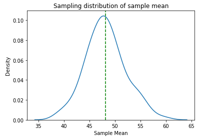
4. Sampling distribution

sns.distplot(sample_means1,hist=False)
plt.title(“Sampling distribution of sample mean”)
plt.axvline(sample_m1.mean(),color=’green’,linestyle=’ — ‘)
plt.xlabel(“Sample Mean”)

The sampling distribution is close to a normal distribution

5. Let’s check the sampling mean and standard error.

print (“Sampling mean: “,round(sample_m1.mean(),2))
print (“Standard Error: “,round(sample_m1.std(),2))
#Output:
Sampling mean:  47.96
Standard Error:  6.39

Standard Error = 6.39. Let’s increase the sample size and check whether the standard error decreases.

6. Take sample size greater than 30 and calculate sampling mean

sample_means2=[]
for i in range(0,100):
 sample=np.random.choice(population1,size=50)
 sample_means2.append(np.mean(sample))

sample_m2=np.array(sample_means2)

7. Sampling distribution

sns.distplot(sample_means2,hist=False)
plt.title(“Sampling distribution of sample mean”)
plt.axvline(sample_m2.mean(),color=’green’,linestyle=’ — ‘)
plt.xlabel(“Sample Mean”)

 

The sampling distribution is normal now.

8. Calculate sampling mean and standard error

print (“Sampling mean: “,round(sample_m2.mean(),2))
print (“Standard Error: “,round(sample_m2.std(),2))

# Output:
Sampling mean:  48.17
Standard Error:  3.89

After increasing the sample size, the standard error decreases. Now the Standard Error is 3.89.

9. Let’s verify our population mean

print (“Population Mean: “,round(population1.mean(),2))

#Output:
Population Mean: 48.03

We have calculated the sampling mean as 48.17 which is approximately equal to the population mean 48.03

10. Calculating Confidence Interval at 99% confidence level.

Lower_limit=sample_m2.mean()- (2.58 * (sample_m2.std()))
print (round(Lower_limit,2))
#Output: 38.14

Upper_limit=sample_m2.mean()+ (2.58 * (sample_m2.std()))
print (round(Upper_limit),2)
#Output: 58.19

Confidence Interval = 38.14 — 58.19

---

Conclusion

In this article, I have covered the central limit theorem, sampling distributions, standard error, and confidence interval. Hope you all like it.

Thanks for reading!

---

Watch this space for more articles on Python and DataScience. If you like to read more of my tutorials, follow me on Medium, LinkedIn, Twitter.