Inferential Statistics for Data Science

---

Basics of Probability, Probability Distributions

Inferential Statistics

Inferential Statistics allows you to make predictions(inferences) from data.

Most often, we will work with a large amount of data for data analysis. So, we will take a sample of data and make predictions/inferences from the sample by using inferential statistics.

But while predicting, we can’t find the exact value. So, we will talk in terms of probability.

---

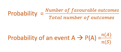
Probability

Probability is the measure of the likelihood that an event will occur. It ranges between o and 1. Higher the probability, the more certain that the event will occur.

Example:
1. Probability of getting 1 while rolling a die is 1/6
2. Probability of getting an even number while rolling a die is 1/2

Probability Terminologies

• Experiment
  An experiment is any well-defined action, that can be infinitely repeated and has a well-defined set of outcomes.
  Example: Tossing a coin, rolling a die.
• Outcome 
  An outcome is defined as any possible results of an experiment. 
  Example: While rolling a die, possible outcomes are 1,2,3,4,5 or 6. 
• Sample Space 
  The set of all possible outcomes in an experiment.
  Example: Rolling a die. S={1,2,3,4,5,6}
• Event 
  An event is the set of favorable outcomes of an experiment. It is a subset is sample space.
  Example: 
  1. An event of getting 1 while rolling a die. E={1}
  2. An event of getting an even number while rolling a die. E={2,4,6}

Mutually Exclusive Events — Addition Rule of Probability

Mutually Exclusive Events 

Two events A and B are said to be mutually exclusive if both events can’t occur at the same time.
Example: Getting a Head or Tail is said to be mutually exclusive. Both events can’t occur at the same time.

Addition Rule 1:

When two events A, B are mutually exclusive, the probability of getting A or B is the sum of the probability of A and the probability of B.

P(A or B) = P(A) + P(B)

Example: From a deck of 52 cards, probability of getting King or Queen.

Probability of getting a King → P(A) = 4/52
Probability of getting a Queen→ P(B) = 4/52

Probability of getting a King or Queen → P(A or B) = 4/52 +4/52 = 8/52
P(A or B) = 2/13

Addition Rule 2:

When two events A, B are not mutually exclusive, the probability of A or B is 

P(A or B) =P(A) +P(B) -P(A ∩B)

Example: From a deck of 52 cards, probability of getting a King or a red card.

Probability of getting a King P(A)=4/52
Probability of getting a red card P(B)=26/52
Probability of getting a red King P(A ∩B)=2/52

Probability of getting a King or red card= 4/52+26/52–2/52 = 28/52

P(A or B) =7/13 

Independent Events — Multiplication Rule of Probability

Independent Events 

Independent events are those events whose occurrence is not dependent on any other event.

Example: Probability of getting 2 heads while tossing 2 coins together. 
The probability of getting a head on one coin is independent on the probability of getting a head on another coin.

P(A and B) =P(A) *P(B)

P((A and B) = 1/2 * 1/2 = 1/4

Dependent Events — Conditional Probability

Dependent events are those events whose occurrence is dependent on any other event. 

P(A and B) =P(A) * P(B |A)

Example: Probability of drawing two kings from the deck of 52 cards.

Probability of choosing a King from the deck of cards P(A) = 4/52

Probability of choosing the second King from the deck of cards P(B|A) = 4/51 

Probability of choosing two kings from the deck of cards = 4/52 * 3/51 = 12/2652

Probability of choosing two kings from the deck of cards = 1/221

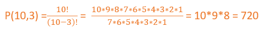
Permutations and Combinations

Permutations

Permutations-Order does matter.

Two types of permutations:

1. Repetition is allowed.

Example: ATM pin number should be four-digit. [Repetition is allowed but the order also matters.] 

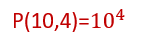
2. Repetition is not allowed.

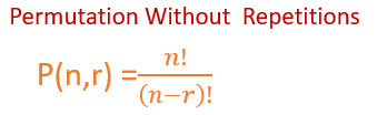
Example: Selecting 3 winners among 10 like first place, second place, and third place. (Order does matter and repetition not allowed)

Combinations

Combinations-Order does not matter.

Two types of combinations:

1. Repetition is allowed.

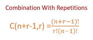
Example: Three flavors of ice-cream are available in that shop. (vanilla,chocolate,strawberry). One person can have only two scoops of ice_cream. What are the different combinations available? 

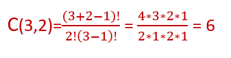
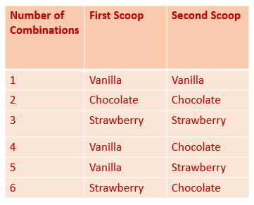
Six different combinations are available.

2. Repetition is not allowed.

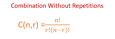
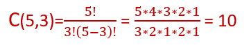
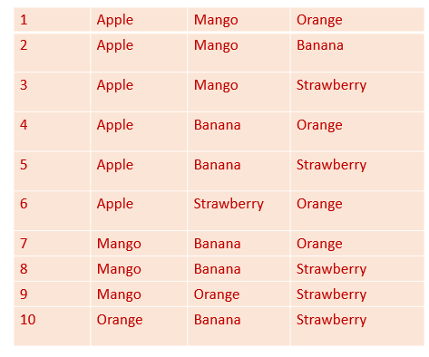
Example: Choosing 3 different fruits from the basket containing 5 different fruits [Order does not matter and repetition not allowed] 
Choosing three from apple, mango, orange, banana, strawberry

---

Probability distributions and Random variable

Random variable

A random variable is the numerical description of the outcome of an experiment.
1. Discrete Random Variable
2. Continuous Random Variable

1. Discrete Random Variable

If a random variable takes a finite number of distinct values or an infinite sequence of values, then it is said to be a discrete random variable.

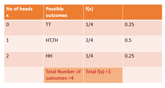
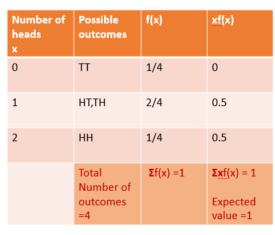
Example: Probability of getting heads when we toss 2 coins?

Here Probability of tossing two coins is an experiment.

The random variable is denoted by X 

“The number of heads” is the random variable.

In this case, X can be 0 head,1 head, or 2 heads

S={HH,HT,TH,TT}

P(X=0) →Probability of getting no head while tossing 2 coins = 1/4
P(X=1) → Probability of getting one head while tossing two coins =2/4
P(X=2) → Probability of getting two head while tossing two coins = 1/4

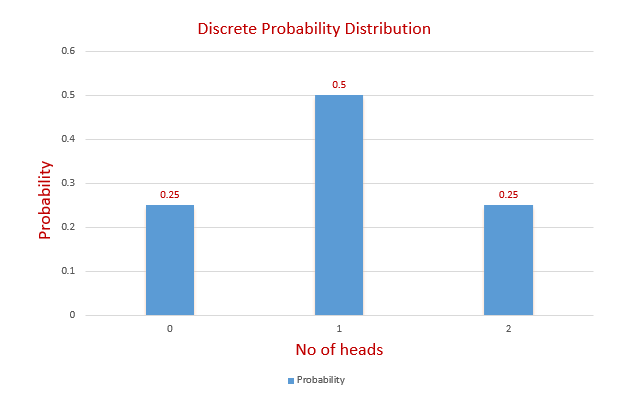
Discrete Probability Distribution

The probability of a random variable describes how the probabilities are distributed over the values of a random variable.

A probability distribution can be represented by an equation or graph.

Equation

The probability distribution is defined by a probability function which is denoted by f(x). It provides the probability for each value of the random variable.
The required conditions of discrete probability function are

f(x)≥0
Σf(x)=1

Graph

Expected Value

The expected value or mean of a random variable is calculated by
E(x)=Σxf(x) = μ

Calculating the expected value of the above example.
Probability of getting heads when we toss 2 coins?

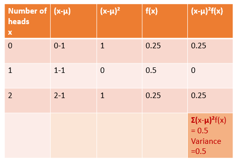
Variance

The variance of a random variable determines the degree to which the values of the random variable varies from the expected value(mean).

The variance of a random variable x is calculated by

Var(x) = σ² =Σ(x-μ)²f(x)

Calculating the variance of the above example

Standard Deviation

Standard deviation is the square root of the variance

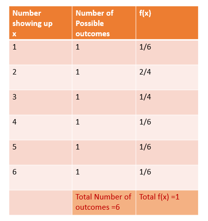
Discrete Uniform Probability Distribution

In discrete uniform probability distribution, the values of the random variables are equally likely.

The discrete uniform probability function is
f(x) = 1/n 
n → number of random variables.

Example: Rolling a dice. All 6 numbers are equally likely.

Binomial Probability Distribution

Properties of Binomial distribution

1. The experiment should contain a sequence of n identical trials.
2. Each trial should have only two outcomes. (like success or failure)
3. The probability of success is denoted as p. It remains fixed for all trials.
4. Each trial is independent.

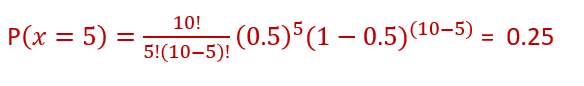
Example: Probability of getting exactly 5 heads while tossing a coin 10 times.

Let’s check whether our example follows the properties of the binomial distribution.

1. It has 10 identical trials
2. It has 2 outcomes. Head / Tail
3. The probability of getting head is p. It remains the same for all trials.
4. Each trial is independent.

Binomial Probability function

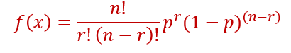
Let’s see how we get this equation.

1. First, we will calculate the total number of combinations of getting r heads in n trials.

2. Then, let’s calculate the probability of getting r heads in n trials.

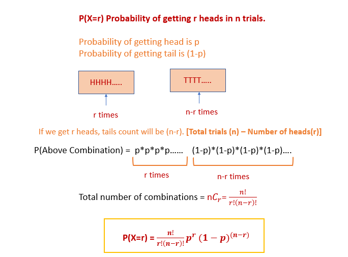
Hence, we get the binomial distribution equation.

Using this formula, let’s calculate the probability of getting exactly 5 heads while tossing a coin 10 times.

Cumulative Probability distribution

In the previous example, we have calculated the probability of the exact value. (exactly 5 heads).

If we need to calculate values like less than 4, or something like that, then the cumulative distribution function is used.

Probability of getting less than 4 heads while tossing a coin 10 times=P(X<4) 

P(X<4)=P(X=0)+P(X=1)+P(X=2)+P(X=3)

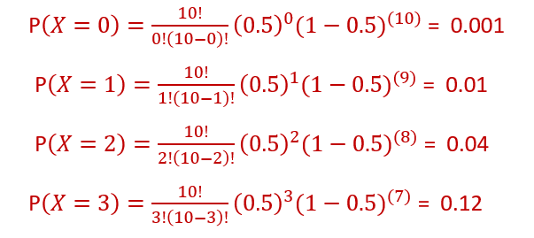
P(X<4)= 0.001+0.01+0.04+0.12 =0.17

Probability of getting less than 4 heads while tossing a coin 10 times =0.17

---

2. Continuous Random Variable

Continuous Random variable takes all value in a certain interval. Continuous Random Variable is usually measurements

Example: Weight of a random student in a class. 

Let’s see about the probability of continuous random variables.

Continuous Probability Distribution 

 We can’t talk about the probability of the continuous random variable for a specific value. But we can find the probability of a continuous random variable in certain intervals.

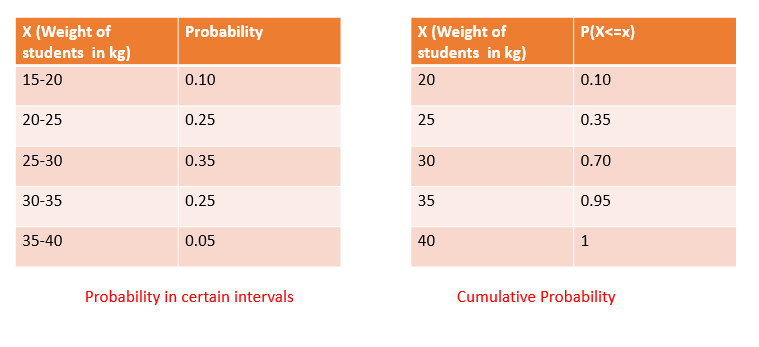
Example: Suppose let’s calculate the probability of weight of students in a class.

Here, we have the probability of a continuous random variable in intervals.

If we want to find the probability of weight of students in class less than 25
P(X≤25), we can find it in two ways.

1. Probability Density Function(PDF)
2. Cumulative Distribution Function (CDF)

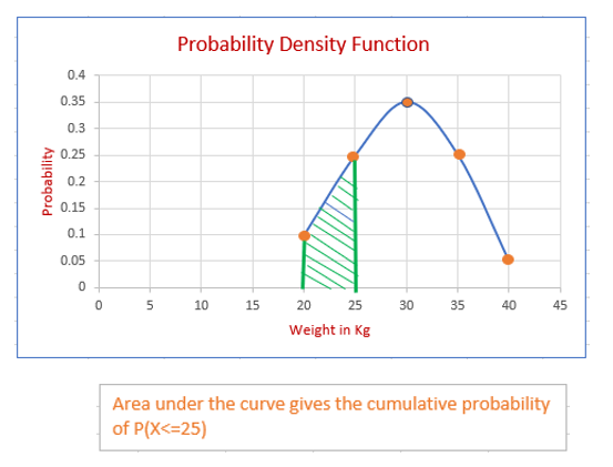
Probability Density Function

Let’s plot the probability of weight in certain intervals.

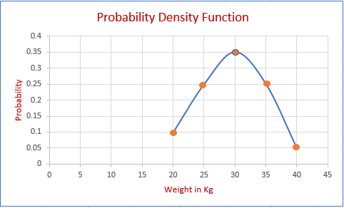
Now, we have to find the probability of weight of students in class less than 25 P(X≤25). In the Probability density function, the area under the curve gives the probability value.

Cumulative Distribution Function

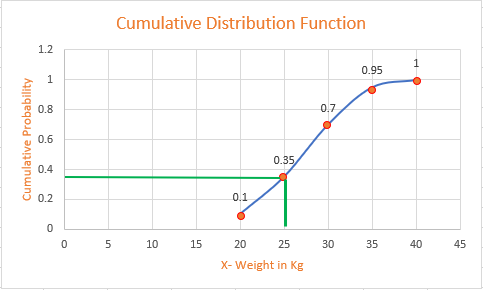
We can find P(X≤25) by using the cumulative probability function. First, let’s calculate cumulative probability.

Let’s plot the cumulative probability of X(weight of students ) vs X (weight of students)

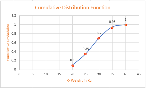
Since, its cumulative function, it will be increasing. The highest value it reaches should be 1. 

Now, from the graph, we can find P(X≤25). The probability of the weight of students less than 25 is 0.35

We can use both PDF and CDF to find the probability distribution of a continuous random variable. PDF is better when compared to CDF. 
In PDF, it’s easier to see patterns. But in CDF, it keeps on increasing.

Normal Probability Distribution

Out of all distribution, Normal Probability Distribution is the most important distribution of a continuous random variable. It is mostly used for statistical inference.

Characteristics of Normal distribution

1. The distribution is symmetric.
2. It has two parameters mean and standard deviation.
3. The highest point of the normal distribution is the mean which is also median and mode.
4. The standard deviation determines the spread of the curve. More the standard deviation, the curve will be wider.
5. The probability of the random variable is measured by the area under the curve.
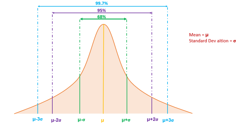
6. It follows the empirical rule also known as the three-sigma rule or 
   68–95–99.7 rule.

• 68% of values of a random variable fall within 1 standard deviation of its mean.
• 95% of values of a random variable fall within 2 standard deviations of its mean.
• 99.7% of values of a random variable fall within 3 standard deviations of its mean.

Standard Normal Distribution

In a normal distribution, to find the probability, we care about the difference between the mean and the value of X. Basically it is the same as how many standard deviations away from the mean.

We can standardize the normal distribution, by converting each value of X to Z(which indicated how many standard deviations away from the mean)

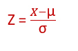
Z is the important parameter in Standard Normal Distribution. Z is unit free.

Suppose if we have Weights of people in kg normally distributed, we will get one normal distribution curve.

If we convert the same weight into lbs means, we will get another normal distribution curve.

So, we can have one curve, by converting X into Z. 

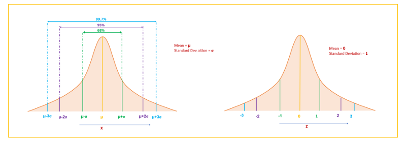
To find the cumulative probability of given Z, we can use the Z table.

A random variable having a normal distribution with a mean of 0 and a standard deviation of 1 is said to have a standard normal distribution.

Conclusion

In this article, I have covered the basics of probability and different probability distributions.

Thanks for reading my article, I hope you found it helpful

---