Everything to Know About Residuals in Linear Regression

Assumptions of linear regression, residuals, Q-Q plot

Residual Analysis in Linear Regression

Assumptions in Linear regression are about residuals. Let’s learn about residuals and assumptions in linear regression about residuals.

Residuals:

Residuals in Linear Regression are the difference between the actual value and the predicted value.

How is the predicted value calculated?

ε → Residuals or Error term.

Assumptions in Linear Regression are about residuals:

1. Residuals should be independent of each other.
2. Residuals should have constant variance.
3. The expected value or mean of the residuals should be zero. E[ε]=0
4. Residuals should follow a normal distribution

Residual Plots

1. Residual vs target variable
2. Residual vs predicted variable
3. Distplot of residuals

Scenario 1: All assumptions are satisfied

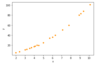
Example: I have taken a simple dataset.

x- independent variable, y-target variable.

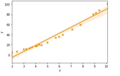
Before building a linear regression model, let’s check scatterplot,regplot, and heatmap.

df=pd.read_csv("ex1.csv")

Scatterplot

sns.scatterplot(df['x'],df['y'],color='darkorange')

regplot

sns.regplot(df['x'],df['y'],color='darkorange')

df.corr()

Building model and calculating residuals

import statsmodels.api as sm
X_train_sm = sm.add_constant(X)
fit1 = sm.OLS(y, X_train_sm).fit()

#Calculating y_predict and residuals

y_predict=fit1.predict(x_train_sm)
residual=fit1.resid

Assumption 1: Residuals are independent of each other.
Assumption 2: Residuals should have a constant variance.

To check these assumptions, we have to plot residual plot [y_predict vs residuals’]

sns.residplot(y_predict,residual,color='darkorange')
plt.xlabel("y_predict")
plt.ylabel("Residuals")
plt.title("Residual Plot")

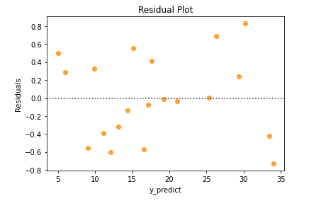
From the above residual plot, we could infer that the residuals didn’t form any pattern. So, the residuals are independent of each other.

And also, the residuals have constant variance. Variance doesn’t seem to increase/decrease constantly with the y_predict value.

Assumption 3: Residuals are normally distributed

To check whether the residuals are normally distributed from Q-Q plot,distplot

1. Q-Q plot → quantile-quantile plot

If the residuals are normally distributed, then the Q-Q plot of residuals will be a straight line

from scipy import stats
import statsmodels.api as sm
residual=fit1.resid

probplot=sm.ProbPlot(residual,stats.norm,fit=True)
fig=probplot.qqplot(line='45')
plt.title('qqplot')

2. distplot

sns.distplot(residual,color='darkorange')

Scenario 2: Residuals are not independent of each other

I have created a small data set that contains x and y and y = x² with some noise added to it.

y →target variable
x →independent variable

1. Scatterplot

df1=pd.read_csv("ex2.csv")
sns.scatterplot(df1['x'],df1['y'],color='darkorange')

1. Regplot

sns.regplot(df1['x'],df1['y'],color='darkorange')

Correlation value

Building Model and calculating y_predict and residuals

X1 = np.array(df1['x']).reshape(-1,1) # predictor variable
y1 = np.array(df1['y']).reshape(-1,1) # response variable
import statsmodels.api as sm
x1_train_sm = sm.add_constant(X1)
fit2 = sm.OLS(y1, x1_train_sm).fit()
y1_predict=fit2.predict(x1_train_sm)
residual_1=fit2.resid

Residual plot

sns.residplot(y1_predict,residual_1,color='darkorange')
plt.xlabel("y1_predict")
plt.ylabel("Residuals")
plt.title("Residual Plot")

From the residual plot, we could see that the residuals follow a pattern. They are dependent on each other. Non-linearity is present in the data.

Since the residuals are dependent on each other, we can now build a slightly different model.

Let’s build a degree 2 polynomial model

from sklearn.preprocessing import PolynomialFeatures
polynomial_features= PolynomialFeatures(degree=2)
xp = polynomial_features.fit_transform(X1)
xp_train=sm.add_constant(xp)
fit_p= sm.OLS(y,xp_train).fit()
yp_predict=fit_p.predict(xp_train)
residual_p=fit_p.resid

Let’s check the residual plot for the new model

sns.residplot(yp_predict,residual_p,color='darkorange')
plt.xlabel("yp_predict")
plt.ylabel("Residuals")
plt.title("Residual Plot")

Now, the residuals are independent of each other.

Scenario 3: Residuals doesn’t have constant variance

If the residuals don’t have constant variance, we can try transforming independent variables (log-transformation,box-cox transformation)

If the residuals don’t have constant variance, we can infer it from the residual plot. If we get a residual plot like the one mentioned below, it means that residuals don’t have constant variance. Here, the residuals spread is not constant.

Conclusion:

In this article, I have covered residuals, the assumptions of residuals in linear regression, and plots to check the assumptions of residuals.

Thanks for reading!

---

If you like to read more of my tutorials on Python and Data Science,
follow me on Medium, Twitter

https://indhumathychelliah.medium.com/membership