Line of Best Fit in Linear Regression

Correlation Coefficient, Coefficient of determination, Model Coefficient

Linear Regression

Linear Regression is one of the most important algorithms in machine learning. It is the statistical way of measuring the relationship between one or more independent variables vs one dependent variable.

The Linear Regression model attempts to find the relationship between variables by finding the best fit line. 
Let’s learn about how the model finds the best fit line and how to measure the goodness of fit in this article in detail

Table of Content

1. Coefficient correlation r
2. Visualizing coefficient correlation
3. Model coefficient → m and c 
   *Slope
   *Intercept
4. Line of Best Fit
5. Cost Function
6. Coefficient of Determination →R² → R-squared
7. Correlation Coefficient vs Coefficient of Determination

---

Simple Linear Regression

Simple Linear Regression is the linear regression model with one independent variable and one dependent variable.

Example: Years of Experience vs Salary, Area vs House Price

Before building a simple linear regression model, we have to check the linear relationship between the two variables.

We can measure the strength of the linear relationship, by using a correlation coefficient.

Correlation Coefficient

It is the measure of linear association between two variables. It determines the strength of linear association and its direction.

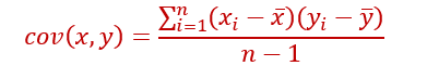
Covariance checks how the two variables vary together.

Covariance depends on units of x and y. Covariance ranges from -∞ to + ∞.
But Correlation coefficient is unit-free. It is just a number.

Coefficient Correlation r ranges from -1 to +1

• If r=0 → It means there is no linear relationship. It doesn’t mean that there is no relationship
• r will be negative if one variable increases, other variable decreases.
• r will be positive, if one variable increases, the other variable also increases.

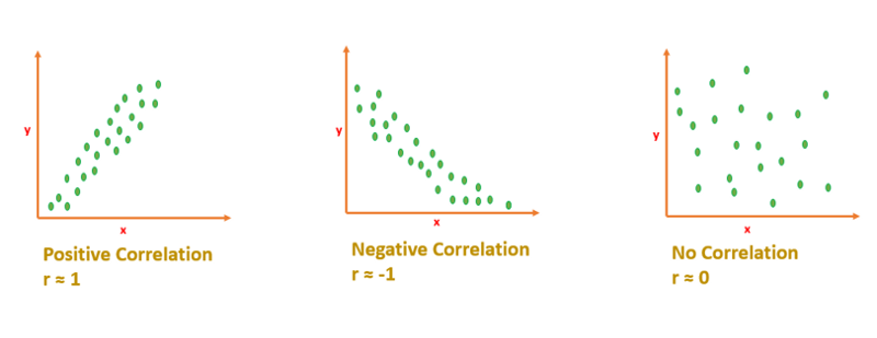
Interpreting Correlation Coefficient

If r is close to 1 or -1 means, x and y are strongly correlated.
If r is close to 0 means, x and y are not correlated. [No linear relationship]

Visualizing Correlation

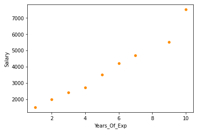
Example: “Years of experience” Vs “Salary”. Here we want to predict the salary for a given ‘Year of experience’.

Salary → dependent variable
Years_of_Experience →Independent Variable.

1. Scatterplot to visualize the correlation

df=pd.read_csv('salary.csv')
sns.scatterplot(x='Years_Of_Exp',y='Salary',data=df,color='darkorange')

2. Exact r value -heatmap

sns.heatmap(df.corr(),annot=True)

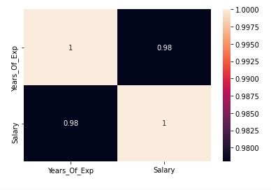
r is 0.98 → It indicates both the variables are strongly correlated.

The Best Fit Line

After finding the correlation between the variables[independent variable and target variable], and if the variables are linearly correlated, we can proceed with the Linear Regression model.

The Linear Regression model will find out the best fit line for the data points in the scatter cloud.

Let’s learn how to find the best fit line.

Equation of Straight Line

y=mx+c

m →slope
c →intercept

Model Coefficient

Slope m and Intercept c are model coefficient/model parameters/regression coefficients.

Slope →m

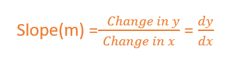
Slope basically says how steep the line is. The slope is calculated by a change in y divided by a change in x

The slope will be negative if one increases and the other one decreases.
The slope will be positive if x increases and y increases.

The value of slope will range from -∞ to + ∞.

[Since we didn’t normalize the value, the slope will depend on units. So, it can take any value from -∞ to + ∞]

Intercept → c

The value of y when x is 0. 
When the straight line passes through the origin intercept is 0.

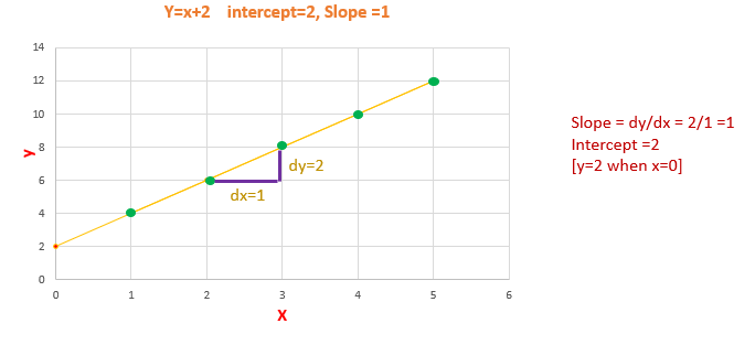
The slope will remain constant for a line. We can calculate the slope by taking any two points in the straight line, by using the formula dy/dx.

Line of Best Fit

The Linear Regression model have to find the line of best fit.

We know the equation of a line is y=mx+c. There are infinite m and c possibilities, which one to chose?

Out of all possible lines, how to find the best fit line?

The line of best fit is calculated by using the cost function — Least Sum of Squares of Errors.

The line of best fit will have the least sum of squares error.

Cost Function

The least Sum of Squares of Errors is used as the cost function for Linear Regression.

For all possible lines, calculate the sum of squares of errors. The line which has the least sum of squares of errors is the best fit line.

Error/Residuals

Error is the difference between the actual value of y and the predicted value of y.

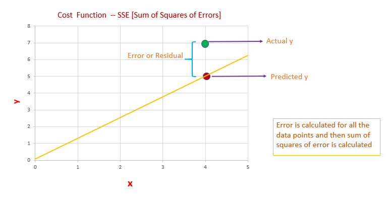
1. We have to calculate error/residual for all data points
2. square the error/residuals.
3. Then we have to calculate the sum of squares of all the errors.
4. Out of all possible lines, the line which has the least sum of squares of errors is the line of best fit.

The reason behind squaring the error/residuals

1. If we are not squaring the error, the negative and positive signs will cancel. We will end up with error=0
2. So we are interested only in the magnitude of the error. How much the actual value deviates from the predicted value.
3. So, why we didn’t consider the absolute value of error. Our motive is to find the least error. If the errors are squared, it will be easy to differentiate between the errors comparing to taking the absolute value of the error.
4. Easier to differentiate the errors, it will be easier to identify the least sum of squares of error.

Out of all possible lines, the linear regression model comes up with the best fit line with the least sum of squares of error. Slope and Intercept of the best fit line are the model coefficient.

Now we have to measure how good is our best fit line?

Coefficient of Determination R² → R-squared

R-squared is one of the measures of goodness of the model. (best-fit line)

SSE →Sum of squares of Errors
SST →Sum of Squares Total

What is the Total Error?

Before building a linear regression model, we can say that the expected value of y is the mean/average value of y. The difference between the mean of y and the actual value of y is the Total Error. 
Total Error is the Total variance. Total Variance is the amount of variance present in the data.

After building a linear regression model, our model predicts the y value. The difference between the mean of y and the predicted y value is the Regression Error.
Regression Error is the Explained Variance. Explained Variance means the amount of variance captured by the model.

Residual/Error is the difference between the actual y value and the predicted y value.
Residual/Error is the Unexplained Variance.

Total Error = Residual Error + Regression Error

Coefficient of determination or R-squared measures how much variance in y is explained by the model.

The R-squared value ranges between 0 and 1

0 → being a bad model and 1 being good.

Key Takeaways

• Correlation Coefficient- r ranges from -1 to +1
• The coefficient of Determination- R² ranges from 0 to 1
• Slope and intercept are model coefficients or model parameters.

Thank you for reading my article, I hope you found it helpful!

https://towardsdatascience.com/the-concepts-behind-logistic-regression-6316fd7c8031

---

Watch this space for more articles on Python and DataScience. If you like to read more of my tutorials, follow me on Medium, LinkedIn, Twitter.

Become a Medium Member by Clicking here: https://indhumathychelliah.medium.com/membership