A Comprehensive Guide to Pandas for Data Science

Quick dive into Pandas

A Comprehensive Guide to Pandas for Data Science

Pandas

Pandas is an open-source python package that provides numerous tools for high-performance data analysis and data manipulation.

Let’s learn about the most widely used Pandas Library in this article.

Table of content

1. Pandas Series
2. Pandas DataFrame
3. How to create Pandas DataFrame?
4. Understanding Pandas DataFrames
5. Sorting Pandas DataFrames
6. Indexing and Slicing Pandas Dataframes
7. Subset DataFrames based on certain conditions
8. How to fill/drop the null values?
9. Lambda functions to modify dataframe
10. Merge, Concatenate dataframes
11. Grouping and aggregating

---

Pandas Datastructures

Pandas supports two datastructures

1. Pandas Series
2. Pandas DataFrame

Pandas Series

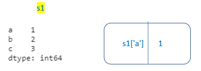
Pandas Series is a one-dimensional labeled array capable of holding any data type. Pandas Series is built on top of NumPy array objects.

 

In Pandas Series, we can mention index labels. If not provided, by default it will take default indexing(RangeIndex 0 to n-1 )

 

Accessing elements from Series.

1. For Series having default indexing, same as python indexing

2. For Series having access labels, same as python dictionary indexing.

How Pandas Series is different from 1-D Numpy Array

1. Pandas Series can hold a variety of data types whereas Numpy supports only numerical data type
2. Pandas Series supports index labels.

Pandas DataFrame

Pandas Dataframe is a two dimensional labeled data structure. It consists of rows and columns.

Each column in Pandas DataFrame is a Pandas Series.

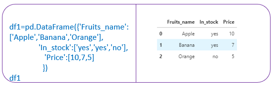
How to Create Pandas DataFrames?

We can create pandas dataframe from dictionaries,json objects,csv file etc.

1. From csv file

2. From a dictionary

3.From JSON object

---

Understanding Pandas DataFrames

 

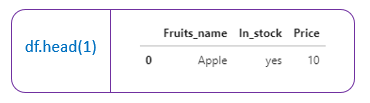
1. df.head() →Returns first 5 rows of dataframe (by default). Otherwise, it returns the first ’n’ rows mentioned.

 

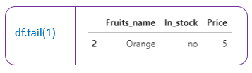
2. df. tail() →Returns the last 5 rows of the dataframe(by default). Otherwise it returns the last ’n’ rows mentioned.

 

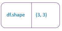
3.df.shape → Return the number of rows and columns of the dataframe.

 

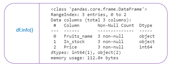
4.df.info() →It prints the concise summary of the dataframe. This method prints information of the dataframe like column names, its datatypes, nonnull values, and memory usage

 

5. df.dtypes() → Returns a series with the datatypes of each column in the dataframe.

 

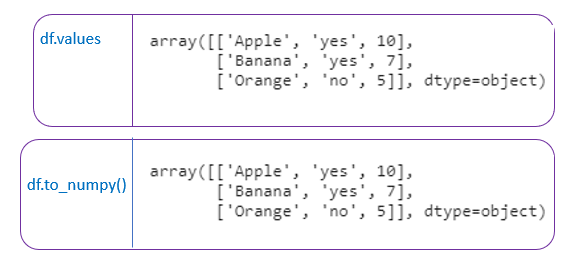
6. df. values → Return the NumPy representation of the DataFrame.
 df.to_numpy() → This also returns the NumPy representation of the dataframe.

 

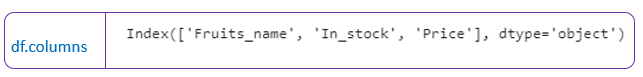
7.df.columns → Return the column labels of the dataframe

8. df. describe() → Generates descriptive statistics. It describes the summary of all numerical columns in the dataframe.
df. describe(include=” all”) → It describes the summary of all columns in the dataframe.

 

 

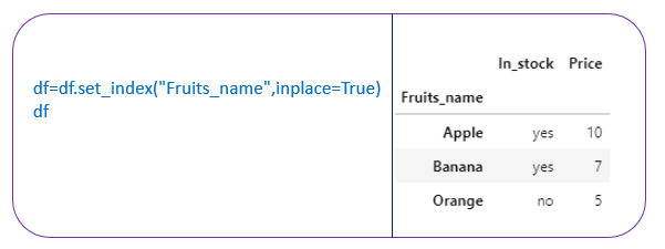
8. df.set_index() → sets the dataframe index using the existing columns. By default it will have RangeIndex (0 to n-1)

df.set_index(“Fruits_name”,inplace=True)
or
df=df.set_index(“Fruits_name”)

[To modify the df, have to mention inplace=True or have to assign to df itself. If not, it will return a new dataframe and the original df is not modified..]

 

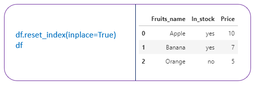
9. df.reset_index() → Reset the index of the dataframe and use the default -index.

 

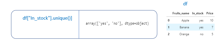
10. df.col_name.unique() → Returns the unique values in the column as a NumPy array.

 

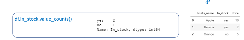
11. df.col_name.value_counts() → Return a Series containing counts of unique values.
Suppose if we want to find the frequencies of the values present in the columns, this function is used.

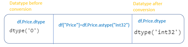
11. df.col_name.astype() → Converting datatype of a particular column.

df.Price.astype(“int32”) → Converting data type of “Price” column to int

---

Sorting dataframe

1. Sorting dataframe by index
2. Sorting dataframe by values

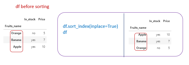
Sorting dataframe by index

1. df.sort_index(ascending=False) → It will sort the row_index in descending order.

 

2. df.sort_index() → It will sort the row_index in ascending order.

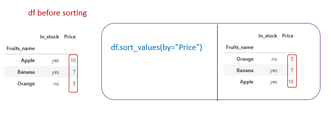
Sorting dataframe by values

1. df.sort_values(by=”Price”) → It will sort the dataframe by column”Price”

---

Indexing and Slicing Pandas DataFrame

1. Standard Indexing
2. Using iloc → Position based Indexing
3. Using loc → Label based Indexing

 

Standard Indexing

1. Selecting rows

Selecting rows can be done by giving a slice of row index labels or a slice of row index position.

df[start:stop]

start,stop → it can be row_index _position or row_index _labels.

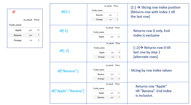
Slice of row index position [End index is exclusive]

df[0:2] → Same as python slicing. Returns row 0 till row 1. 
df[0:6:2] → Returns row 0 till row 5 with step 2. [Every alternate rows]

Slice of row index values [End index is inclusive]

df[“Apple”:] →Returns row “Apple” till the last row in the dataframe
df[“Apple”:” Banana”] → Returns row “Apple” till row “Banana”.

 

Note:

• We can’t explicitly mention row index position or row index labels. It will raise a keyError.
  df[“Banana”] 
df[1]
Both will raise KeyError.
• We have to mention only the slice of row index labels/row index position.
• Selecting rows will return a dataframe.

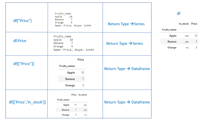
2. Selecting columns

We can select a single column in two ways. Selecting a single column will return a series.
1.df[“column_name”]
2. df.column_name

If a single column_name is given inside a list, it will return a dataframe. 
df[[“column_name”]]

To select multiple columns, have to mention a list of column_names

df[[“column_name1”,”column_name2"]]

Selecting multiple columns will return a dataframe.

 

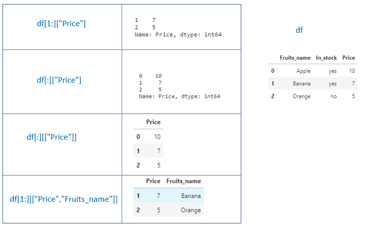
3. Selecting rows and columns

Selecting rows and columns can be given by

df[start:stop][“col_name”]

df[start:stop][[“col_name”]]

If we mention a single column, it will return a series.
If we mention single column/multiple columns in a list, it will return a dataframe.

 

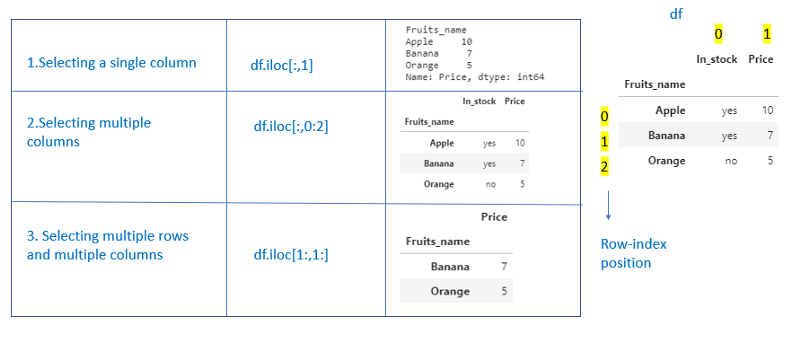
Using iloc -Integer based Indexing.

Using iloc, we can index dataframes using index position

df[row_index_pos,col_index_pos]

row_index_pos → It can be a single row_index position, a slice of row index_ position, list of row_index_position. 
This field is mandatory

col_index_pos → It can be a single col_index_position, slice of col_index_position or list of col_index_position.
This field is optional. If not provided, by default, it takes all columns.

1.Selecting rows

 

2. Selecting columns

 

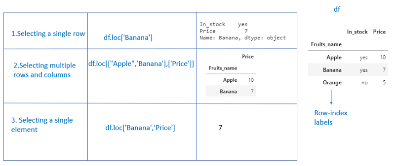
Using loc

Using loc, we can index dataframes using labels.

df.loc[row_index_labels,col_index_labels]

row_index_labels can be a single row_index label, a slice of row_index label, or a list of row_index labels.
This field is mandatory.

col_index_labels can be a single col_index label, a slice of col_index_label, or a list of col_index labels.
This field is optional. If not provided, by default, it takes all columns.

[If the dataframe has default indexing, then row_index_position and row_index labels will be the same]

1. Dataframe not having default indexing

 

2. Dataframe having default indexing

 

---

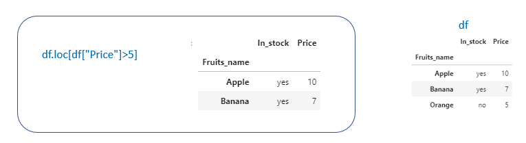
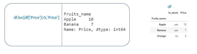
Subset dataframe based on certain conditions

In Pandas, we can subset dataframe based on certain conditions.

Example. Suppose we want to select rows having “Price” > 5
df[“Price”]>5 will return a booelan array

We can pass this boolean array inside df. loc or standard indexing
[df. iloc means we have to remember the column_index position]

 

 

---

How to drop/ fill the null values in the dataframe

Suppose we want to check whether pandas dataframe has null values.

df.isnull().sum() → Returns the sum of null values in each column in the df

df[“col_name”].isnull().sum() → Returns the sum of null values for that particular column in the df.

If we want to look into the rows which have null values

df[df[“Price”].isnull()] → Returns the row which has null values in the “Price” column.

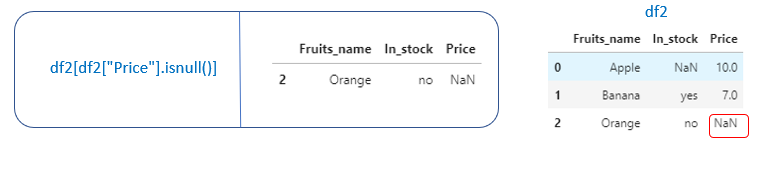
After looking into the rows, we can decide whether to drop or fill the null values.

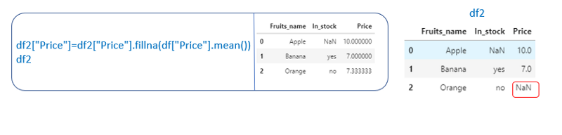
If we want to fill the null values with a mean value

df[“col_name”].fillna(df[“col_name”].mean())

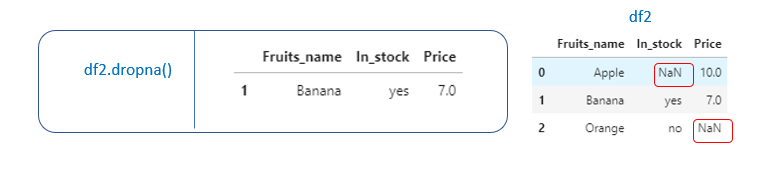
If we want to drop the rows having a null value.

1. To drop the rows having null values in a particular column
   df.dropna(subset=[“col_name”])

 

2. To drop all the rows having null values
df.dropna()

 

To modify the original df, have to mention inplace=True or have to assign it to the original df itself.

3. Specify the boolean condition to drop the null values.

---

Lambda Functions to modify a column in the dataframe

Suppose if the columns in our dataframe are not in the correct format means, we need to modify the column. We can apply lambda functions on a column in a dataframe using the apply() method.

Example 1: Let’s check the columns and datatypes of the columns in the dataframe (df.dtypes).

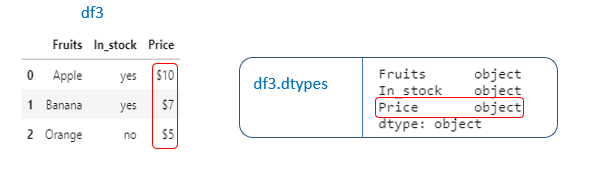
“Price” column is in object datatype. We need to change it to int data type so that we can perform mathematical operations.

“Price” column has $ symbol laso. We need to remove that and then convert it to int datatype.

Have to write lambda functions to remove the $ sign and to convert it to int datatype

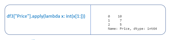
lambda x: int(x[1:]) → This lambda function will remove $ sign (which is in index 0 in the “Price” column) and convert it to int datatype.

Let’s apply this lambda function using apply() method on “Price” column

df3[“Price”].apply(lambda x: int(x[1:]))

To modify the original dataframe, we can assign it to the “Price” column

df3[“Price”]=df3[“Price”].apply(lambda x: int(x[1:]))

 

Example 2: If we have null values in the “Price” column and we have replaced that null values with the mean value.

We can see that the “Price” column having float numbers with many decimal places.

Now, using the lambda function, we can round it to two decimal places.

---

Merge, Concat DataFrames

Sometimes, we need to merge/ concatenate multiple dataframes, since data comes in different files.

Merging Dataframes

pd.merge() → Used to merge multiple dataframes using a common column.

Example. Let’s see different ways to merge the two dataframes.

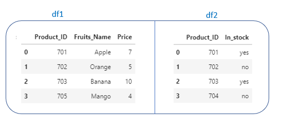
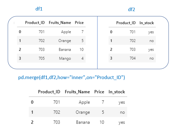
We have “Product_ID” in common in both dataframes. Let’s merge df1 and df2 on “Product_Id”.

1. inner

pd.merge(df1,df2,how=”inner”,on=”Product_ID”) →It will create a dataframe containing columns from both df1 and df2. Merging happens based on values in column “Product_ID”

inner → similar to an intersection or SQL inner join. It will return only the common rows in both the dataframes.

 

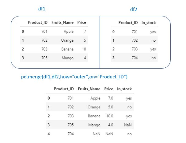
2. outer

pd.merge(df1,df2,how=”outer”,on=”Product_ID”)

outer → Similar to union/SQL full outer join. It will return all the rows from both dataframe.

 

3. left

pd.merge(df1,df2,how=”left”,on=”Product_ID”)

left → Returns all rows from left df. Here left df = df1

 

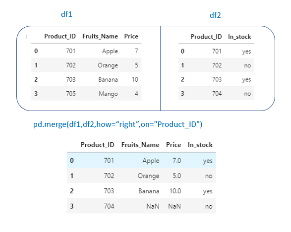
4. right

pd.merge(df1,df2,how=”right”,on=”Product_ID”)

right → Returns all rows from left df. Here right df = df2

 

Concatenate Dataframes

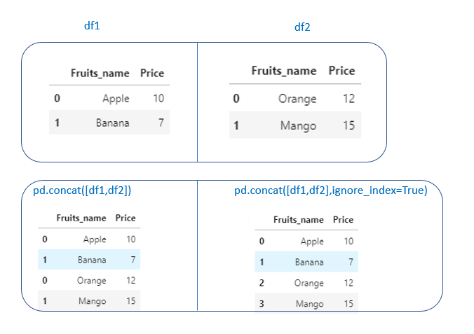
pd.concat() → It will concatenate two dataframes on top of each other or side by side.

Mostly, this can be used when we want to concatenate two dataframes having the same columns

Example:

pd.concat([df1,df2]) → It will concatenate df1 and df2 on top of each other.
pd.concat([df1,df2],ignore_index=True) → If we want to ignore the index column, set ignore_index=True.

---

Grouping and Aggregating

In pandas, groupby operation involves three steps.

1. Splitting the data into groups based on some criteria.
2. Applying a function to each group( Ex. sum(),count(),mean() ..)
3. Combines the result into a data structure like DataFrame.

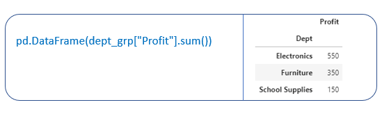
Example: We want to calculate the total profit of each dept.

 

First, we have to do groupby() on Dept column.
Then we have to apply the aggregate function → sum() on that group

1. Creating groupby object on “Dept”

Typically, we will group the data using a categorical variable.

dept_grp=df1.groupby("Dept")
dept_grp

Output: <pandas.core.groupby.generic.DataFrameGroupBy object at 0x048DA238>

df.groupby() returns a groupby object.

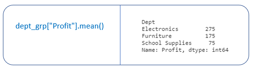
2. Applying aggregate function on groupby object.

The aggregation function returns a single aggregate value for each of the groups.
In our example, we have “Electronics”,” Furniture” and “School Supplies” groups.

 

 

3. Combine the results into a DataStructure

---

Conclusion

In this article I have covered some basic pandas functionality like how to do indexing, sorting, filtering, merging, concatenating, grouping, and aggregating pandas dataframes. And also how to do data cleaning like dropping null values and data manipulation by applying some function on a column.

I hope I have covered some basic Pandas functionality. Thank you for reading my article, I hope you found it helpful!

---

My blog on Numpy

View at Medium.com

---

Watch this space for more articles on Python and DataScience. If you like to read more of my tutorials, follow me on Medium, LinkedIn, Twitter.