Linear Regression in Python

The math behind Linear Regression and the Python way of implementation

Linear Regression in Python

Linear Regression is a machine learning algorithm based on supervised learning. Linear Regression is a predictive model that is used for finding the linear relationship between a dependent variable and one or more independent variables. Here,dependent variable/target variable(Y) should be continuous variable.

Let’s learn the math behind simple linear regression and the Python way of implementation using ski-kit learn

Dataset

Let’s looks at our dataset first. I have taken a simple dataset for an easy explanation. Years of Experience vs Salary.

We want to predict the salary of the person based on their years of experience?

Math Behind the Simple Linear Regression

Dataset

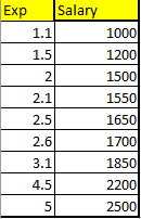
In the given dataset, we have Exp vs Salary. Now, we want to predict the salary for 3.5 years of experience? Let’s see how to predict that?

Linear Equation

c →y-intercept → What is the value of y when x is zero?
The regression line cuts the y-axis at the y-intercept.

Y → Predicted Y value for the given X value

Let’s calculate m and c.

m is also known as regression co-efficient. It tells whether there is a positive correlation between the dependent and independent variables. A positive correlation means when the independent variable increases, the mean of the dependent variable also increases.

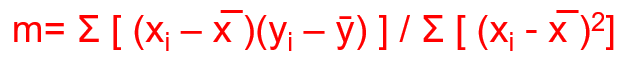
The Regression coefficient is defined as the covariance of x and y divided by the variance of the independent variable, x.

Variance → How far each number in the dataset is from the mean.
x̄ → mean of x
ȳ → mean of y

Covariance →It’s a measure of the relationship between two variables.

I have done all the math calculations in an excel sheet which can be downloaded from my GitHub link.

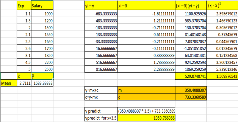
Covariance =( Σ [ (xi — x̅ )(yi — ȳ) ])/n=529.0740741

Variance =(Σ [ (xi — x̅ )²])/n= 1.509876543

m= Covariance /Variance =529.0740741/1.509876543=350.4088307

m=350.4088307

Now to calculate intercept c

y=mx+c
c=y-mx
Apply mean y (ȳ) and mean x (x̅)in the equation and calculate c

c= 1683.33333-(350.4088307*2.7111)
c=733.3360589

After calculating m and c, now we can do predictions.

Let’s predict the salary of a person having 3.5 years of experience.

y=mx+c
m=350.4088307
c=733.3360589

y predict = (350.4088307 * 3.5) + 733.3360589 = 1959.766966

The predicted y value for x=3.5 is 1959.766966

Performance Evaluation

To evaluate how good our regression model is, we can use the following metrics.

SSE-Sum of Squares Error

The error or residual is the difference between the actual value and the predicted value. The sum of all errors can cancel out since it can contain negative signs and give zero. So, we square all the errors and sum it up. The line which gives us the least sum of squared errors is the best fit.

The line of best fit always goes through x̅ and ȳ.

In Linear Regression, the line of best fit is calculated by minimizing the error(the distance between data points and the line).

Sum of Squares Errors is also known as Residual error or Residual sum of squares

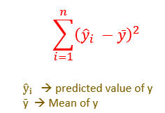
SSR Sum of Squares due to Regression

SSR is also known as Regression Error or Explained Error.
It is the sum of the differences between the predicted value and the mean of the dependent variable ȳ

SST Sum of Squares Total

SST/Total Error = Sum of squared errors + Regression Error.

Total Error or Variability of the data set is equal to the variability explained by the regression line (Regression Error) plus the unexplained variability (SSE) known as error or residuals.

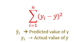
Explained Error or Variability → SSR
Unexplained Error → SSE

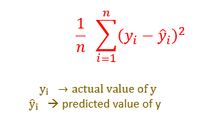
MSE → Mean Squared Error

MSE is the average of the squared difference between the actual and predicted values of the data points.

RMSE -Root Mean Squared Error

RMSE is a measure of how spread out these residuals are. In other words, it tells you how concentrated the data is around the line of best fit.
RMSE is calculated by taking the square root of MSE.

Interpretation of RMSE:
RMSE is interpreted as the standard deviation of unexplained variance(MSE).
RMSE contains the same units as the dependent variable.
Lower values of RMSE indicates a better fit.

Coefficient of Correlation (r)

Before building the model, have to identify good predictors. The coefficient of Correlation (r) is used to determine the strength of the relationship between two variables. It will help to identify good predictors.

Formula:

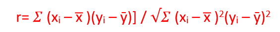
The value of r range from -1 to 1.
-1 indicates a negative correlation which means when x increases y decreases.
+1 indicates a positive correlation which means both x and y travels in the same direction.
0 or close to 0 means no correlation.

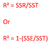
R²( R square )→ Coefficient of determination

The coefficient of determination → This metric is used after building the model, to check how reliable the model is.

R² →It is equal to the variance explained by regression (Regression Error or SSR) divided by Total variance in y (SST)

R² → It describes how much of the total variance in y is explained by our model.
If Error(unexplained error or SSE)<Variance (SST) means the model is good.
The best fit is the line in which unexplained error (SSE) is minimized.

R² values range from 0 to 1.

0 → indicates Poor model
1 or close to 1 → indicates the Best model

Calculating MSE, RMSE, R² in our dataset

---

Let’s do the same implementation in Python using scikit learn.

The code used can be downloaded as a Jupyter notebook in my GitHub link.

1.Import the libraries needed

import numpy as np
import pandas as pd
import matplotlib.pyplot as plt
import seaborn as sns

2. Load the data

df=pd.read_csv("exp1.csv")
df

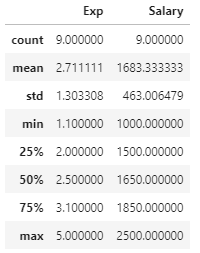
df.describe()

3. EDA — Exploratory Data Analysis

• Scatterplot

plt.scatter(df.Exp,df.Salary,color='red')

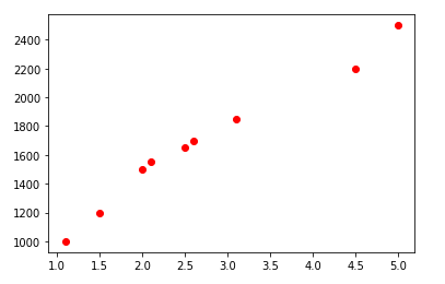
[We can find linear relationship between x and y]

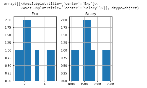
• Histogram

df.hist()

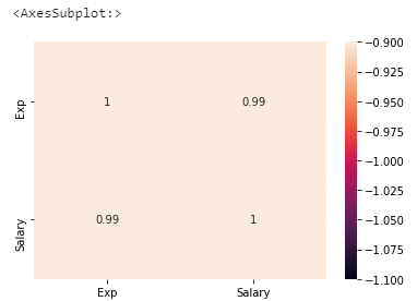
• Finding the Coefficient of Correlation (r)

df.corr()

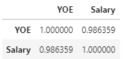
r value 0.98 indicates a strong relationship.

We can plot correlation using the heatmap

sns.heatmap(df.corr(),annot=True,vmin=-1,vmax=-1)

• Finding missing values

df.isna().sum()

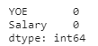
[No Missing values are there]

4. Assign Features to X and Y

x=df.iloc[:,0:1]
x.head(1)

y=df.iloc[:,1:]
y.head(1

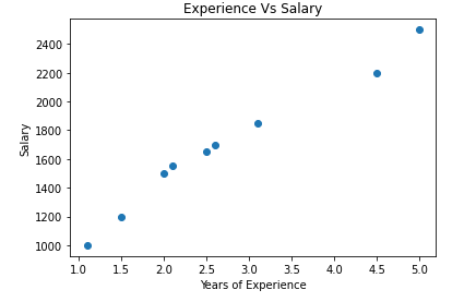
5. Visualize the dataset

plt.scatter(x, y)
plt.title('Experience Vs Salary')
plt.xlabel('Years of Experience')
plt.ylabel('Salary')
plt.show()

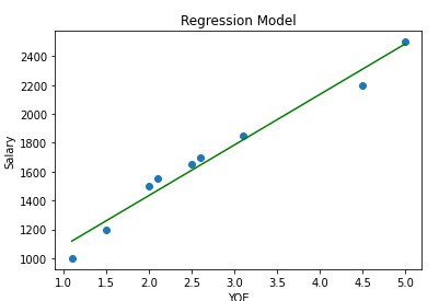
6. Model Building with sklearn

from sklearn.linear_model import LinearRegression
lin_reg=LinearRegression()
lin_reg.fit(x,y)

Visualize the model

plt.scatter(x,y)
plt.plot(x,lin_reg.predict(x),color='green')
plt.title("Regression Model")
plt.xlabel("YOE")
plt.ylabel("Salary")

7. Predict the salary for 3.5 years of experience using the model

ypredict=lin_reg.predict(np.array([[3.5]]))
ypredict
#Output:array([[1959.76696648]])

8. m (slope) and c(intercept) values

lin_reg.coef_
#Output:array([[350.40883074]])
lin_reg.intercept_
#Output:array([733.33605887])

9. Calculate the coefficient of determination

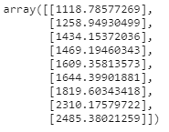
ypredict=lin_reg.predict(x)
ypredict

from sklearn.metrics import mean_squared_error,r2_score,explained_variance_score
print ("Coefficient of determination :",r2_score(y,ypredict))
print ("MSE: ",mean_squared_error(y,ypredict))
print("RMSE: ",np.sqrt(mean_squared_error(y,ypredict)))

#Output:
Coefficient of determination : 0.9729038186936964
MSE:  5163.327882256747
RMSE:  71.85630022661024

We get the same values using math calculation and python implementation.
If it’s a large dataset, we have to split the data for training and testing.

GitHub Link

Code, dataset, excel sheet used in this story is available in my GitHub Link

Conclusion

In this story, we have taken the simple dataset and learned the math behind simple linear regression and python way of implementation using scikit learn.
We can also implement linear regression using statsmodel.

My other blogs on Machine learning

Understanding Decision Trees in Machine Learning

Logistic Regression in Python

Naive Bayes Classifier in Machine Learning

An Introduction to Support Vector Machine

An Introduction to K-Nearest Neighbors Algorithm

---

Thanks for reading!